Best practices for your confirmatory factor analysis
A JASP and lavaan tutorial
Author
Affiliation
Pablo Rogers
Universidade Federal de Uberlândia
Published
March 13, 2024
Abstract
This supplementary material provides the complete R/lavaan implementation for the confirmatory factor analysis (CFA) tutorial presented in Rogers (2024). The analyses use the WHOQOL-BREF instrument — a 24-item quality of life measure covering four domains: Psychological, Physical, Social, and Environment — with data from a Brazilian sample of 1,047 respondents (Rogers, 2021). The codes that generates the outputs for this tutorial article can be found in the notebook: https://phdpablo.github.io/cfa-brm/index-preview.html
A central challenge in applied CFA is that items are typically measured on ordinal Likert scales, yet many textbooks and software default to Maximum Likelihood (ML) estimation, which assumes continuous, multivariate normal data. As discussed in Rogers (2024), the appropriate approach for ordinal data is the Diagonally Weighted Least Squares (DWLS) estimator — implemented as WLSMV in lavaan — which operates on polychoric correlations rather than Pearson correlations and does not assume normality of observed variables.
ImportantTutorial Structure
This document is organized as a manuscript project: the Article presents the analytical narrative and results without showing code, while the Article Notebook displays the full R code behind every result. Both views share the same content — the only difference is code visibility.
2 Setup
We begin by loading all required R packages. The lavaan package provides the core CFA estimation engine; semTools extends it with reliability functions and additional diagnostics; semPlot produces path diagrams; psych provides descriptive statistics and omega coefficients for bifactor models; simsem enables Monte Carlo simulation for power analysis; and dynamic computes the Dynamic Fit Index (DFI) cutoffs.
In [1]:
library(lavaan)
This is lavaan 0.6-21
lavaan is FREE software! Please report any bugs.
O seguinte objeto é mascarado por 'package:psych':

    Holzinger
library(dplyr)
Anexando pacote: 'dplyr'
O seguinte objeto é mascarado por 'package:MASS':

    select
Os seguintes objetos são mascarados por 'package:stats':

    filter, lag
Os seguintes objetos são mascarados por 'package:base':

    intersect, setdiff, setequal, union
library(ggplot2)
Anexando pacote: 'ggplot2'
Os seguintes objetos são mascarados por 'package:psych':

    %+%, alpha
We set global options and a seed for reproducibility. The seed ensures that all simulation-based results (power analysis) are exactly reproducible.
In [2]:
options(max.print =1000000)set.seed(123456)
NoteA Note on Code Design
Throughout this tutorial, you will notice that some code patterns are repeated across sections — for example, extracting fit indices, formatting factor loadings, and building comparison tables. In a production environment, these routines would typically be modularized into reusable R functions and sourced from separate scripts.
We deliberately chose not to do this. Each analysis section is self-contained, with all code written explicitly and in sequence. This design sacrifices automation and conciseness in favor of transparency: the reader can follow each step without navigating between files or tracing function definitions. For a tutorial whose primary goal is to teach CFA best practices, we believe clarity of exposition is more valuable than code elegance.
Readers who wish to adapt this workflow for their own research are encouraged to refactor repeated patterns into functions and organize them into modular scripts — this is, in fact, a best practice for reproducible research projects.
3 Step 1: ETL — Extract, Transform, Load
The WHOQOL-BREF dataset is loaded directly from the Mendeley Data repository (Rogers, 2021). The data file contains N = 1,047 observations with 24 items. A separate label file provides the variable names following the naming convention: item number followed by a suffix indicating its domain (_P = Psychological, _F = Physical, _S = Social, _A = Environment). Items Q3, Q4, and Q26 have already been reverse-coded in the source data so that higher values consistently indicate better quality of life.
Table 2 presents the descriptive statistics for all 24 items. Means range from approximately 3.0 to 4.0, with standard deviations around 0.8–1.1, indicating moderate variability across items. No floor or ceiling effects are evident, and skewness values are generally within acceptable bounds (|sk| < 1), supporting the use of polychoric correlations. These statistics are consistent with the original validation study (Rogers, 2024).
In [6]:
knitr::kable(describe(df0), digits =2)
In [7]:
Table 2: Descriptive statistics for all WHOQOL-BREF items
vars
n
mean
sd
median
trimmed
mad
min
max
range
skew
kurtosis
se
Q3_F
1
1047
4.17
0.93
4
4.31
1.48
1
5
4
-0.99
0.27
0.03
Q4_F
2
1047
4.10
1.01
4
4.26
1.48
1
5
4
-1.02
0.31
0.03
Q10_F
3
1047
3.61
0.91
4
3.65
1.48
1
5
4
-0.18
-0.43
0.03
Q15_F
4
1047
4.42
0.79
5
4.57
0.00
1
5
4
-1.52
2.41
0.02
Q16_F
5
1047
3.50
1.03
4
3.49
1.48
2
5
3
-0.13
-1.16
0.03
Q17_F
6
1047
3.72
0.92
4
3.78
0.00
2
5
3
-0.51
-0.53
0.03
Q18_F
7
1047
3.75
0.96
4
3.81
1.48
2
5
3
-0.50
-0.64
0.03
Q5_P
8
1047
3.29
0.82
3
3.35
1.48
1
5
4
-0.44
-0.09
0.03
Q6_P
9
1047
3.90
0.99
4
4.02
1.48
1
5
4
-0.88
0.48
0.03
Q7_P
10
1047
3.61
0.86
4
3.66
1.48
1
5
4
-0.53
0.12
0.03
Q11_P
11
1047
3.82
0.99
4
3.92
1.48
1
5
4
-0.62
-0.09
0.03
Q19_P
12
1047
3.72
0.95
4
3.77
1.48
2
5
3
-0.42
-0.70
0.03
Q26_P
13
1047
3.91
0.92
4
4.03
0.00
1
5
4
-1.19
1.68
0.03
Q20_S
14
1047
3.64
0.89
4
3.67
1.48
2
5
3
-0.25
-0.66
0.03
Q21_S
15
1047
3.46
1.00
4
3.45
1.48
2
5
3
-0.05
-1.09
0.03
Q22_S
16
1047
3.58
0.88
4
3.60
1.48
2
5
3
-0.16
-0.69
0.03
Q8_A
17
1047
2.94
0.98
3
2.97
1.48
1
5
4
-0.11
-0.43
0.03
Q9_A
18
1047
3.47
0.91
4
3.52
1.48
1
5
4
-0.64
0.26
0.03
Q12_A
19
1047
3.45
1.10
3
3.50
1.48
1
5
4
-0.25
-0.54
0.03
Q13_A
20
1047
3.93
0.82
4
3.98
1.48
1
5
4
-0.57
0.15
0.03
Q14_A
21
1047
3.34
0.96
3
3.34
1.48
1
5
4
-0.29
-0.26
0.03
Q23_A
22
1047
3.98
0.97
4
4.09
1.48
2
5
3
-0.70
-0.45
0.03
Q24_A
23
1047
3.73
0.97
4
3.79
1.48
2
5
3
-0.40
-0.79
0.03
Q25_A
24
1047
3.83
0.98
4
3.91
1.48
2
5
3
-0.50
-0.72
0.03
NoteData Overview
The dataset contains N = 1047 observations on 24 variables. All items are measured on a 5-point Likert scale (1–5), representing ordinal data. This ordinal nature is fundamental: it requires the use of polychoric correlations and DWLS estimation rather than Pearson correlations and ML.
4 Population Model
Before fitting CFA models to our sample data, we define a population model that serves two purposes: (1) computing Dynamic Fit Index (DFI) cutoffs tailored to this specific model structure and sample size, and (2) conducting a priori power analysis via simulation.
The population model is based on the meta-analytic factor loadings from Lin & Yao (2022), who validated the WHOQOL-BREF factor structure using a meta-analysis of exploratory factor analyses combined with social network analysis. Factor correlations were set at 0.3, reflecting the upper bound reported in Lin & Yao (2022) (range 0.08–0.30). Residual variances were derived analytically as 1 − λ² (except for Q3 and Q4, whose residuals are adjusted for their predicted correlation).
Given the ordinal nature of the variables, we assume equidistant thresholds following a linearity assumption with proportions of approximately 12%, 23%, 31%, 23%, and 12%. For a five-point Likert scale, this translates to threshold values of −1.2, −0.4, 0.4, and 1.2. While it is unlikely that thresholds from previous studies will be available, if response frequencies per category per item are provided, thresholds can be estimated using the inverse normal distribution.
ImportantImportant Caveat
This population model should be understood as a teaching illustration. The loadings from Lin & Yao (2022) come primarily from exploratory factor analysis studies using principal components with varimax rotation — a method that has well-known limitations (Rogers, 2022). Ideally, one should seek a robust national survey that has employed CFA with ordinal data for the WHOQOL-BREF, providing more appropriate starting values.
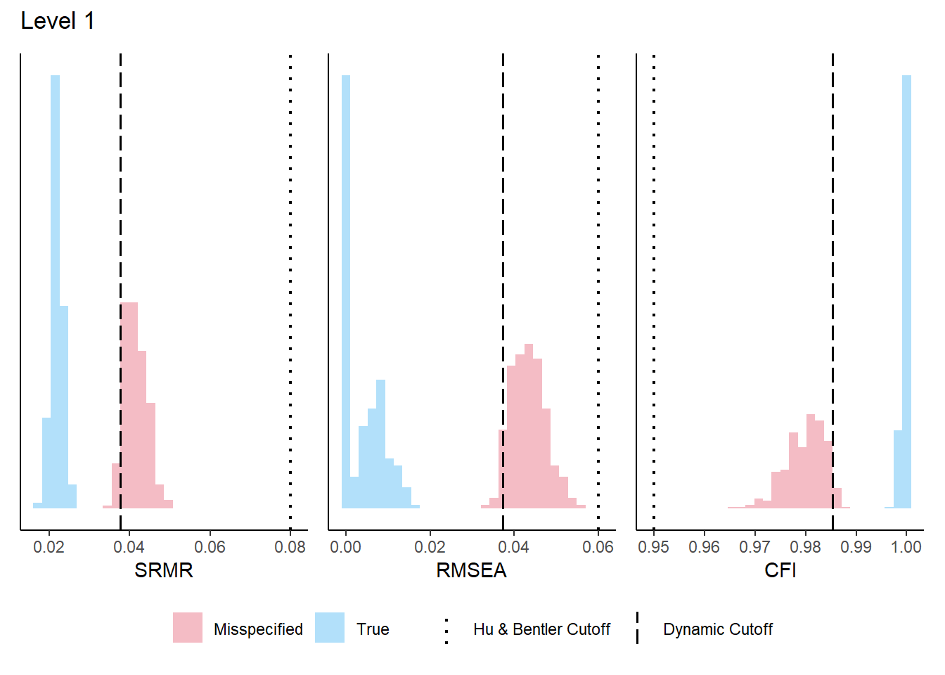
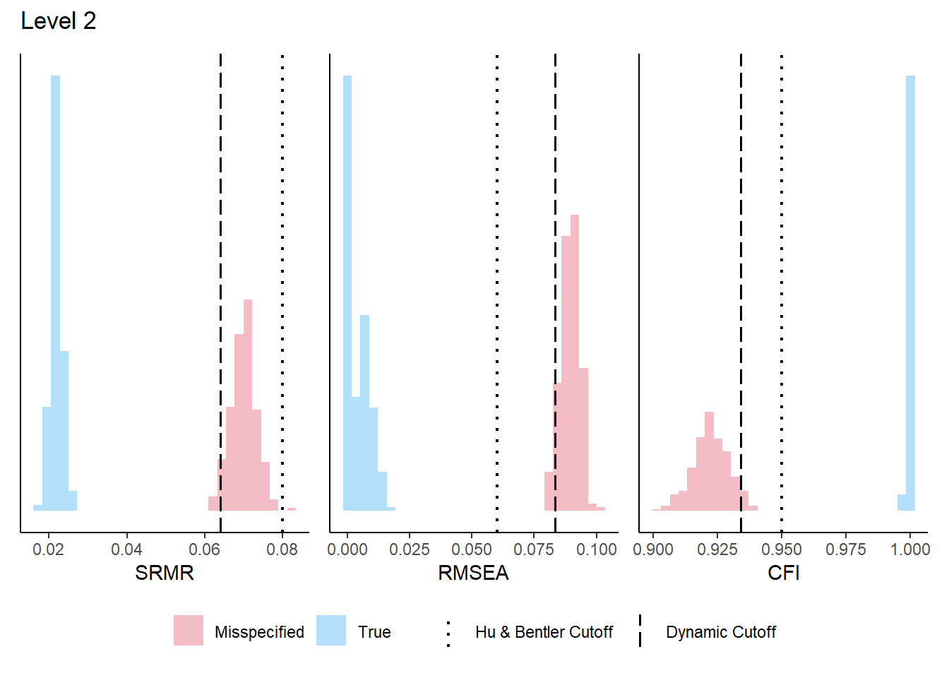
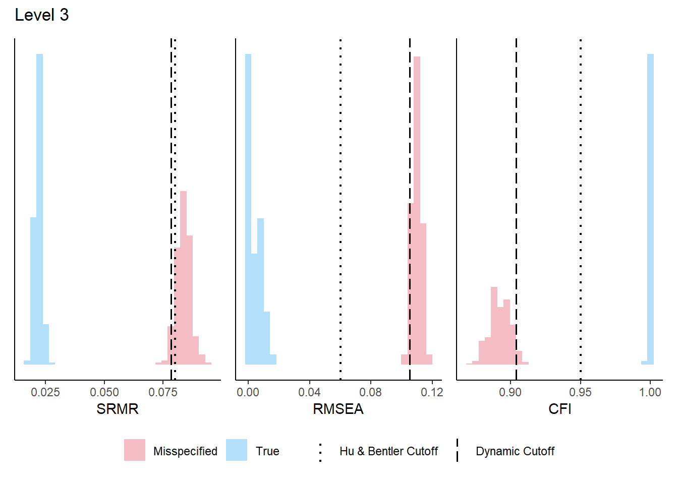
The Dynamic Fit Index (McNeish, 2023) provides simulation-based cutoff values for fit indices that are tailored to a specific model structure and sample size, rather than relying on generic rules of thumb (e.g., CFI > .95, RMSEA < .06). The DFI computation requires the population model defined above.
In [9]:
dynamic::catHB(pop_model, manual =TRUE, n =1047, plot =TRUE)
Warning: lavaan->lavaanify():
   variances of ordered variables are ignored when parameterization =
   "delta"; please remove them from the model syntax or use parameterization
   = "theta"; variables involved are: Q5_P Q6_P Q7_P Q11_P Q19_P Q26_P Q10_F
   Q15_F Q16_F Q17_F Q18_F Q20_S Q21_S Q22_S Q8_A Q9_A Q12_A Q13_A Q14_A
   Q23_A Q24_A Q25_A
Warning: Using `size` aesthetic for lines was deprecated in ggplot2 3.4.0.
ℹ Please use `linewidth` instead.
ℹ The deprecated feature was likely used in the dynamic package.
  Please report the issue at <https://github.com/melissagwolf/dynamic/issues>.
Your DFI cutoffs:
            SRMR  RMSEA CFI   Magnitude
Level-0     0.024 0.012 0.998 NONE
Specificity 95%   95%   95%

Level-1     0.038 0.037 0.985 0.37
Sensitivity 95%   95%   95%

Level-2     0.064 0.083 0.934 0.599
Sensitivity 95%   95%   95%

Level-3     0.078 0.105 0.904 0.58
Sensitivity 95%   95%   95%

 Notes:
  -Number of levels is based on the number of factors in the model
  -'Sensitivity' is % of hypothetically misspecified models correctly identified by cutoff in DFI simulation
  -Cutoffs with 95% sensitivity are reported when possible
  -If sensitivity is <50%, cutoffs will be supressed

 The distributions for each level are in the Plots tab
[[1]]
[[2]]
[[3]]
Note that we could compute a separate DFI for each estimated model (assuming each in turn as the population model). However, this would sacrifice comparability across models. Moreover, DFI methods for bifactor models are not yet available, and those for hierarchical models are still in development.
5 4-Factor CFA Model
The first model tested is the standard four correlated factor model, which represents the theoretical structure of the WHOQOL-BREF (Lin & Yao, 2022).
5.1 Model Specification
Each of the 24 items loads on exactly one of the four latent factors: Psychological (6 items), Physical (7 items), Social (3 items), and Environment (8 items). Latent factors are allowed to freely correlate, reflecting the expected interrelations among quality of life domains. A residual covariance between items Q3 and Q4 is included based on prior theoretical and empirical evidence, as both items assess related aspects within the Physical domain.
The estimation uses DWLS (WLSMV in lavaan) with all items declared as ordinal (ordered = TRUE), and factor variances are fixed to 1 (std.lv = TRUE) for identification.
When evaluating a CFA model, watch for: (1) Heywood cases — standardized loadings > 1 or negative variance estimates, which indicate estimation problems; (2) Overall fit — SRMR < .08, RMSEA < .06, CFI/TLI > .95 using the scaled versions for WLSMV (For reference only, as the correct approach would be to use the cutoffs derived from the DFI); (3) Local fit — standardized residuals > |2|, and modification indices (MI) > 3.84; (4) Reliability — GLB and composite reliability (omega) should exceed .70 for adequate internal consistency.
Table 5: Factor correlations for the 4-factor model
Factor 1
Factor 2
r
SE
p
psycho
physical
0.909
0.010
< .001
psycho
social
0.771
0.019
< .001
psycho
environment
0.725
0.021
< .001
physical
social
0.638
0.024
< .001
physical
environment
0.630
0.022
< .001
social
environment
0.550
0.028
< .001
TipFull lavaan output
For the complete lavaan output — including unstandardized estimates, thresholds, variance parameters, and R² values — run the following command in your R console after fitting the model:
This produces a comprehensive printout that is useful for diagnostic purposes but too extensive for publication. The key results have been extracted into the tables above.
Examining the output, the scaled chi-square test is statistically significant (expected for large N), but this alone is not informative for model evaluation. The scaled fit indices reveal a mediocre fit: the CFI and TLI values fall slightly below the conventional .95 threshold, and the RMSEA exceeds .06. The SRMR is within acceptable range. This pattern is consistent with a Level 2 misspecification according to DFI standards — the model captures the general structure but has notable local misfits.
Regarding factor loadings, most items show adequate standardized loadings (Std.all > .50), indicating substantial association with their respective factors. However, Q4 (Physical) shows a relatively lower loading, and the R² values for Q4 (Physical) and Q24 (Environment) are notably low, suggesting these items are not well-explained by their assigned factor.
5.3.1 Modification Indices
Modification indices (MI) estimate the expected decrease in the chi-square statistic if a currently fixed parameter were freed. An MI > 3.84 is statistically significant at α = .05, and practically relevant MIs typically exceed 10. However, not all high MIs should be acted upon — only those with theoretical justification.
Table 6: Top 20 modification indices for the 4-factor model
lhs
op
rhs
mi
epc
289
Q5_P
~~
Q14_A
177.218
0.278
254
environment
=~
Q5_P
175.788
0.503
544
Q24_A
~~
Q25_A
124.552
0.282
216
physical
=~
Q5_P
119.025
-1.039
467
Q17_F
~~
Q18_F
92.645
0.162
263
environment
=~
Q15_F
89.086
0.347
214
psycho
=~
Q24_A
80.033
-0.333
231
physical
=~
Q24_A
78.731
-0.289
200
psycho
=~
Q10_F
55.182
0.631
265
environment
=~
Q17_F
48.628
-0.251
266
environment
=~
Q18_F
44.622
-0.236
280
Q5_P
~~
Q17_F
44.099
-0.193
281
Q5_P
~~
Q18_F
41.613
-0.188
258
environment
=~
Q19_P
37.766
-0.254
428
Q10_F
~~
Q18_F
34.964
-0.123
252
social
=~
Q24_A
33.765
-0.206
203
psycho
=~
Q17_F
33.378
-0.549
394
Q3_F
~~
Q15_F
32.487
0.181
212
psycho
=~
Q14_A
31.896
0.221
223
physical
=~
Q21_S
30.562
0.233
The modification indices reveal a critical finding: item Q5 appears in multiple high-MI entries, suggesting cross-loadings on factors other than Psychological. This is a strong empirical signal that Q5 may not function as intended within the four-factor structure. Additionally, several MIs suggest correlated residuals between items across domains, reflecting the high correlation between Physical and Psychological factors.
WarningRed Flag: Item Q5
When a single item appears repeatedly among the highest modification indices, this suggests a systematic misfit rather than isolated local strain. Freeing individual parameters (e.g., adding cross-loadings) is generally not recommended as a post hoc strategy — it risks capitalizing on sample-specific patterns. The better approach is to evaluate whether the item should be removed from the model.
5.3.2 Residual Correlations
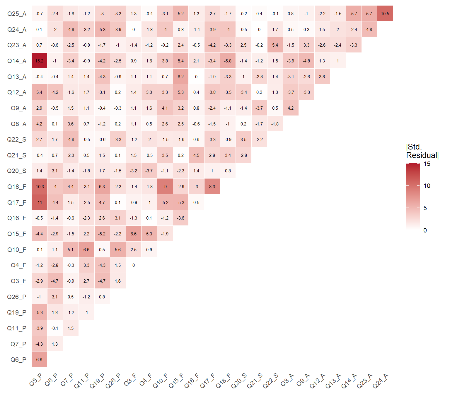
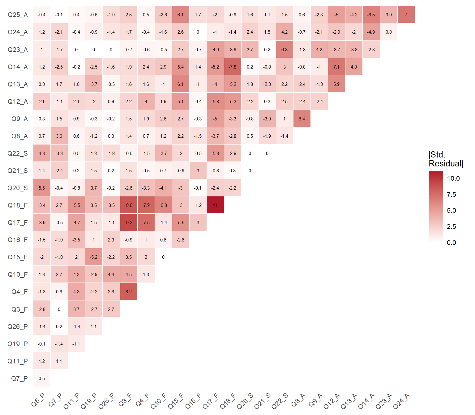
Standardized residuals greater than |2| indicate item pairs whose empirical correlation is poorly reproduced by the model. The correlation residuals below show the discrepancies between model-implied and observed correlations.
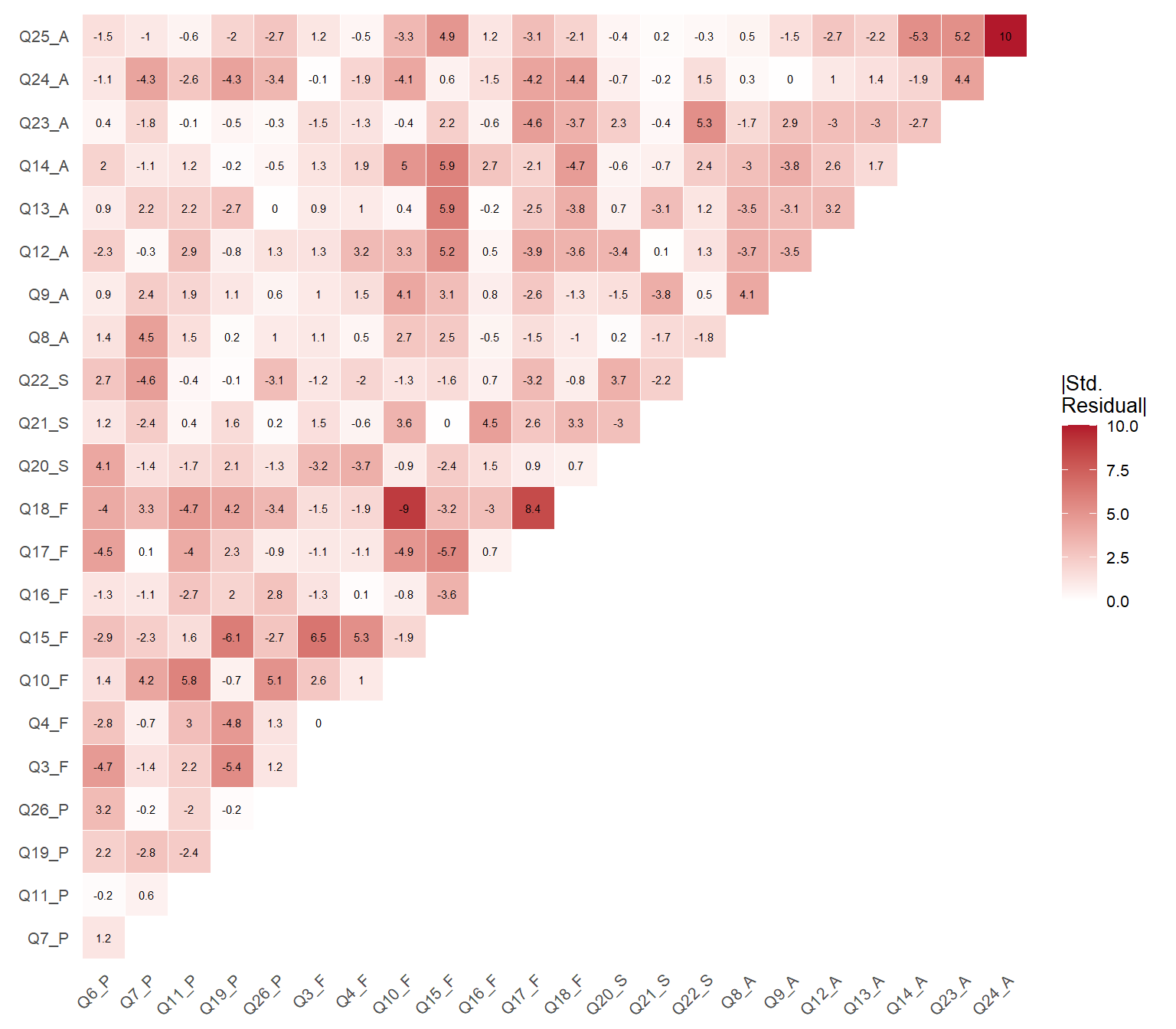
Figure 1: Heatmap of standardized residual correlations for the 4-factor model
Figure 1 provides a global view of local misfit. Color intensity reflects the absolute magnitude of standardized residuals — darker red indicates poorer reproduction of that pairwise correlation by the model, regardless of direction. Cell labels retain the sign: positive values indicate the model underestimates the correlation, negative values indicate overestimation. Pairs exceeding |2| deserve closer inspection.
The residual analysis confirms the patterns identified by the modification indices: the largest standardized residuals involve Q5 and items from other domains, reinforcing the conclusion that this item introduces systematic misfit.
TipFull residual matrices
For the complete residual matrices — including the correlation residuals and the full 24×24 standardized residual matrix — run the following commands in your R console after fitting the model:
residuals(est_4fa, type ="cor")residuals(est_4fa, type ="standardized")$cov
The first command returns the difference between observed and model-implied correlations. The second returns standardized residuals, where values exceeding |2| indicate item pairs whose association is poorly reproduced by the model. The table and heatmap above summarize the most relevant results from these matrices.
5.3.3 Reliability Coefficients
We compute reliability using semTools::reliability(), which provides: alpha (Cronbach’s), omega (composite reliability, preferred for CFA), omega2 (Bentler’s), omega3 (McDonald’s), and AVE (average variance extracted). AVE > .50 indicates that the factor captures more variance from its items than is due to measurement error.
Warning in semTools::reliability(est_4fa):
The reliability() function was deprecated in 2022 and will cease to be included in future versions of semTools. See help('semTools-deprecated) for details.

It is replaced by the compRelSEM() function, which can estimate alpha and model-based reliability in an even wider variety of models and data types, with greater control in specifying the desired type of reliability coefficient (i.e., more explicitly choosing assumptions).

The average variance extracted should never have been included because it is not a reliability coefficient. It is now available from the AVE() function.
For constructs with categorical indicators, Zumbo et al.`s (2007) "ordinal alpha" is calculated in addition to the standard alpha, which treats ordinal variables as numeric. See Chalmers (2018) for a critique of "alpha.ord" and the response by Zumbo & Kroc (2019). Likewise, average variance extracted is calculated from polychoric (polyserial) not Pearson correlations.
In [22]:
Table 7: Reliability coefficients for the 4-factor model
psycho
physical
social
environment
alpha
0.820
0.823
0.687
0.787
alpha.ord
0.854
0.863
0.741
0.820
omega
0.821
0.801
0.707
0.794
omega2
0.821
0.801
0.707
0.794
omega3
0.823
0.811
0.723
0.797
avevar
0.504
0.500
0.524
0.375
All four domains show composite reliability (omega) above .70, indicating adequate internal consistency. The AVE values are acceptable for most domains, with the Environment domain showing a slightly lower value — consistent with its broader and more heterogeneous item content. The Social domain, despite having only three items, shows strong reliability due to the high factor loadings of Q20, Q21, and Q22.
5.3.4 Preliminary Evaluation Summary
Based on the overall and local fit analysis:
Overall fit is mediocre, compatible with a Level 2 misspecification (DFI)
Local indices indicate: (a) high correlation between Physical and Psychological factors (suggesting potential hierarchical structure);
low factor loadings for Q4 and Q24; (c) item Q5 is systematically problematic — it appears in many high MIs and contributes to local misfit
Reliability is adequate for all domains
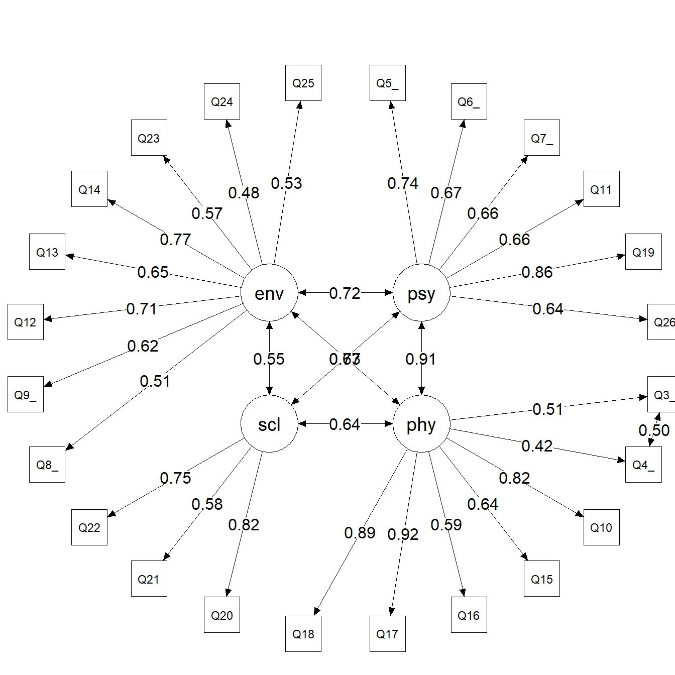
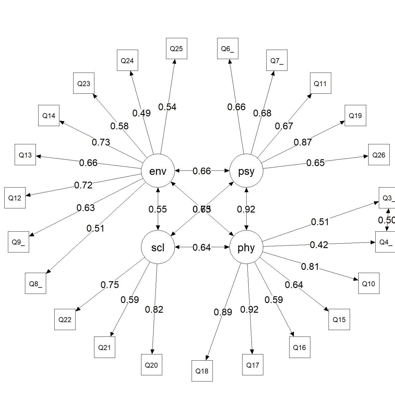
5.4 Path Diagrams
The path diagram below visualize the estimated model. Latent factors are shown as ovals, observed items as rectangles, and standardized factor loadings as edge labels. The circle layout better displays interfactor correlations.
NoteLayout Note
Consider this layout for educational purposes, as for your article you should create something better formatted, which will almost always be done by hand.
Figure 2: Path diagram of the 4-factor CFA model (circle layout)
The circle layout in Figure 2 reveals the strong correlations among all four factors, particularly between Psychological and Physical domains. This pattern motivates the exploration of bifactor and second-order models in the following sections.
6 4-Factor Bifactor Model
Given the high interfactor correlations observed in the 4-factor model, a bifactor structure is a natural alternative. In a bifactor model, a general factor (here, overall Quality of Life — QOL) loads directly on all items alongside specific group factors for each domain. The critical assumption is that all factors — general and specific — are orthogonal (uncorrelated).
This model tests whether there is a meaningful general QOL construct underlying all items, and how much unique variance remains in each specific domain after accounting for the general factor. Item Q5 is excluded from this model due to convergence problems, which further supports the preliminary evidence that Q5 is problematic.
NoteOn Bifactor Models
Bifactor models have gained popularity in psychometrics because they often provide better fit indices than correlated-factor models. However, as discussed in Rogers (2024), some authors argue that this improved fit is partly an artifact of the greater number of parameters, and that the orthogonality assumption rarely holds in practice. These considerations will be important when comparing models.
6.1 Model Specification
In bifactor model syntax, the general factor must be specified first. The Q3–Q4 residual correlation is no longer needed because both items now load on the general factor, which absorbs their shared variance.
Table 9: Standardized factor loadings for the bifactor 4-factor model
Factor
Item
Std.Loading
SE
p
QOL
Q6_P
0.632
0.022
< .001
QOL
Q7_P
0.668
0.019
< .001
QOL
Q11_P
0.666
0.020
< .001
QOL
Q19_P
0.851
0.012
< .001
QOL
Q26_P
0.634
0.022
< .001
QOL
Q3_F
0.422
0.030
< .001
QOL
Q4_F
0.349
0.031
< .001
QOL
Q10_F
0.785
0.014
< .001
QOL
Q15_F
0.584
0.027
< .001
QOL
Q16_F
0.573
0.023
< .001
QOL
Q17_F
0.875
0.012
< .001
QOL
Q18_F
0.842
0.013
< .001
QOL
Q20_S
0.598
0.021
< .001
QOL
Q21_S
0.452
0.026
< .001
QOL
Q22_S
0.541
0.024
< .001
QOL
Q8_A
0.372
0.028
< .001
QOL
Q9_A
0.454
0.026
< .001
QOL
Q12_A
0.499
0.024
< .001
QOL
Q13_A
0.461
0.025
< .001
QOL
Q14_A
0.527
0.024
< .001
QOL
Q23_A
0.380
0.029
< .001
QOL
Q24_A
0.246
0.031
< .001
QOL
Q25_A
0.328
0.029
< .001
psycho
Q6_P
0.696
0.479
0.146
psycho
Q7_P
0.059
0.051
0.247
psycho
Q11_P
0.021
0.032
0.502
psycho
Q19_P
0.085
0.066
0.2
psycho
Q26_P
0.135
0.102
0.184
physical
Q3_F
0.690
0.042
< .001
physical
Q4_F
0.606
0.039
< .001
physical
Q10_F
0.116
0.030
< .001
physical
Q15_F
0.290
0.037
< .001
physical
Q16_F
0.059
0.037
0.107
physical
Q17_F
0.268
0.031
< .001
physical
Q18_F
0.257
0.031
< .001
social
Q20_S
0.566
0.052
< .001
social
Q21_S
0.269
0.035
< .001
social
Q22_S
0.567
0.052
< .001
environment
Q8_A
0.300
0.032
< .001
environment
Q9_A
0.386
0.029
< .001
environment
Q12_A
0.485
0.026
< .001
environment
Q13_A
0.453
0.028
< .001
environment
Q14_A
0.441
0.028
< .001
environment
Q23_A
0.468
0.029
< .001
environment
Q24_A
0.603
0.028
< .001
environment
Q25_A
0.518
0.027
< .001
The bifactor model shows improved fit compared to the original 4-factor model, with slightly better CFI, TLI, and RMSEA values. However, the improvement is modest and the fit remains in the mediocre range (Level 2 of DFI).
Examining the standardized loadings, the general QOL factor captures substantial variance from most items. Notably, the Psychological specific factor shows very low loadings — most of the variance that was previously attributed to the Psychological domain is now absorbed by the general factor. This pattern suggests that psychological well-being items are primarily indicators of overall QOL rather than a distinct domain.
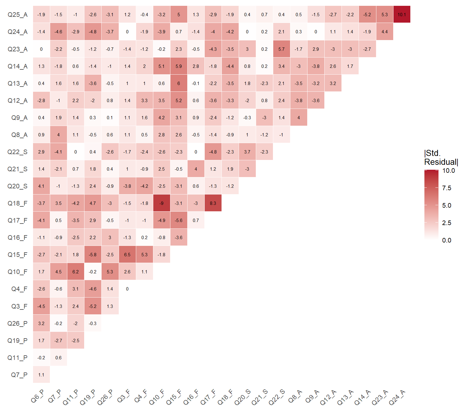
Figure 3: Heatmap of standardized residual correlations for the bifactor 4-factor model
6.3.1 Reliability
For bifactor models, omega from psych::omegaFromSem() provides the most appropriate reliability decomposition: omega hierarchical (ωH) estimates the proportion of total score variance attributable to the general factor, while omega subscale (ωS) estimates the proportion attributable to each specific factor after controlling for the general factor.
The omega hierarchical value indicates that the general QOL factor accounts for a substantial proportion of reliable variance. The Psychological specific factor contributes very little unique reliable variance beyond the general factor, confirming the pattern observed in the loadings. The Physical, Social, and Environment specific factors retain more meaningful unique variance.
6.3.2 Preliminary Evaluation Summary
Overall fit has improved but remains mediocre (Level 2 of DFI, although not directly comparable)
The general (G) factor is statistically relevant and explains substantial variance across all items
The Psychological specific factor loses most of its importance — its variance is almost entirely captured by the general QOL factor
The orthogonality assumption required for this model is a strong restriction that may not hold empirically
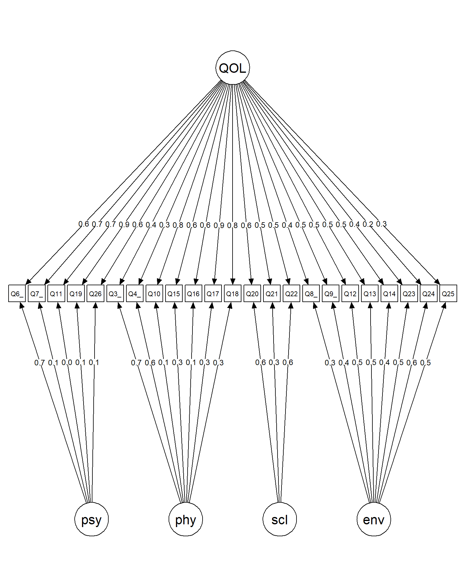
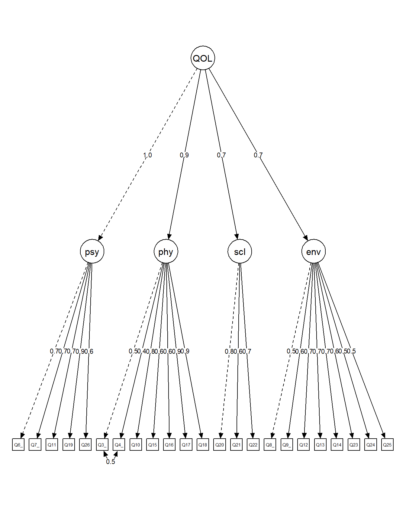
6.4 Path Diagram
The tree3 layout is specifically designed for bifactor diagrams, placing the general factor centrally and specific factors on the sides.
You can test other formatting parameters (edge.label.cex, label.cex, edge.label.position, etc) to simulate path diagrams with better layouts.
7 Second-Order CFA Model
An alternative to the bifactor model is the second-order (hierarchical) model. Here, the general QOL factor does not load directly on items. Instead, it loads on the four first-order factors, which in turn load on the observed items. This structure implies that the influence of the general factor on individual items is mediated by the domain-specific factors — a conceptually different interpretation from the bifactor model.
7.1 Model Specification
Item Q5 is excluded for comparability with the bifactor model. A technical requirement is that the Psychological factor variance must be fixed to zero for model convergence (empirical underidentification), suggesting that essentially all Psychological domain variance is explained by the higher-order QOL factor.
Fixing the Psychological factor variance to zero (psycho ~~ 0*psycho) is necessary for model convergence. This is not merely a technical trick — it has substantive meaning: nearly all variance in the Psychological domain is captured by the general QOL factor. This finding is consistent with the bifactor results, where the Psychological specific factor had minimal importance.
7.2 Model Estimation
Note that std.lv is not used here because the second-order structure imposes its own identification constraints through the higher-order factor loadings.
The second-order model fit is comparable to the other models, though the convergence issue with the Psychological domain is a notable limitation. The second-order loadings (QOL → first-order factors) reveal the relative contribution of each domain to overall quality of life.
Figure 5: Heatmap of standardized residual correlations for the 2nd order 4-factor model
7.3.1 Reliability
For the first-order factors, we use semTools::reliability(). For the second-order QOL factor, semTools::reliabilityL2() provides the appropriate decomposition.
Warning in semTools::reliability(est_4f_2or):
The reliability() function was deprecated in 2022 and will cease to be included in future versions of semTools. See help('semTools-deprecated) for details.

It is replaced by the compRelSEM() function, which can estimate alpha and model-based reliability in an even wider variety of models and data types, with greater control in specifying the desired type of reliability coefficient (i.e., more explicitly choosing assumptions).

The average variance extracted should never have been included because it is not a reliability coefficient. It is now available from the AVE() function.
For constructs with categorical indicators, Zumbo et al.`s (2007) "ordinal alpha" is calculated in addition to the standard alpha, which treats ordinal variables as numeric. See Chalmers (2018) for a critique of "alpha.ord" and the response by Zumbo & Kroc (2019). Likewise, average variance extracted is calculated from polychoric (polyserial) not Pearson correlations.
In [45]:
Table 14: Reliability coefficients for first-order factors (second-order model)
Warning in semTools::reliabilityL2(est_4f_2or, "QOL"):
The reliabilityL2() function was deprecated in 2022 and will cease to be included in future versions of semTools. See help('semTools-deprecated) for details.

It is replaced by the compRelSEM() function, which can estimate alpha and model-based reliability in an even wider variety of models and data types, with greater control in specifying the desired type of reliability coefficient (i.e., more explicitly choosing assumptions).
In [47]:
Table 15: Second-order factor (QOL) reliability
omegaL1
omegaL2
partialOmegaL1
0.838
0.899
0.926
The second-order QOL factor shows adequate reliability, indicating that the four first-order domains collectively serve as reliable indicators of overall quality of life. First-order reliability values remain consistent with those observed in the standard 4-factor model.
Figure 6: Path diagram of the second-order CFA model
8 4-Factor Model Without Item Q5
The analyses above converged on a consistent finding: item Q5 is problematic. It appeared in multiple high modification indices in the original 4-factor model, caused convergence problems in the bifactor model, and its removal was necessary for comparability across alternative models. This is a common scenario in applied CFA — items that appear sound from a content validity perspective may not perform well empirically in a given sample or cultural context.
8.1 Model Specification
This section presents the revised 4-factor model excluding Q5, retaining the correlated residuals between Q3 and Q4. This model will serve as the basis for the final model comparison and post hoc power analysis.
Table 18: Factor correlations for the 4-factor model (Q5 excluded)
Factor 1
Factor 2
r
SE
p
psycho
physical
0.922
0.010
< .001
psycho
social
0.755
0.019
< .001
psycho
environment
0.659
0.024
< .001
physical
social
0.638
0.024
< .001
physical
environment
0.630
0.022
< .001
social
environment
0.550
0.028
< .001
After removing Q5, the overall fit shows improvement. All remaining items exhibit adequate standardized loadings, and the model converges without issues. The Q5 removal resolves the most prominent source of local misfit identified in the original 4-factor model.
Table 19: Top 20 modification indices for the 4-factor model (Q5 excluded)
lhs
op
rhs
mi
epc
510
Q24_A
~~
Q25_A
114.934
0.273
252
environment
=~
Q15_F
94.407
0.351
433
Q17_F
~~
Q18_F
84.659
0.157
222
physical
=~
Q24_A
78.505
-0.281
206
psycho
=~
Q24_A
77.213
-0.289
254
environment
=~
Q17_F
43.449
-0.232
255
environment
=~
Q18_F
42.877
-0.228
192
psycho
=~
Q10_F
42.388
0.704
208
physical
=~
Q6_P
36.087
-0.700
242
social
=~
Q24_A
33.243
-0.203
394
Q10_F
~~
Q18_F
31.926
-0.118
360
Q3_F
~~
Q15_F
31.211
0.178
214
physical
=~
Q21_S
31.008
0.235
198
psycho
=~
Q21_S
26.547
0.277
509
Q23_A
~~
Q25_A
23.889
0.140
415
Q15_F
~~
Q13_A
21.582
0.146
376
Q4_F
~~
Q15_F
21.431
0.147
416
Q15_F
~~
Q14_A
20.568
0.143
480
Q22_S
~~
Q23_A
18.885
0.131
224
social
=~
Q6_P
18.702
0.220
The modification indices are notably reduced compared to the original model. While some MIs remain above 3.84, they are smaller in magnitude and do not show the systematic pattern of misfit associated with Q5.
Warning in semTools::reliability(est_4fb):
The reliability() function was deprecated in 2022 and will cease to be included in future versions of semTools. See help('semTools-deprecated) for details.

It is replaced by the compRelSEM() function, which can estimate alpha and model-based reliability in an even wider variety of models and data types, with greater control in specifying the desired type of reliability coefficient (i.e., more explicitly choosing assumptions).

The average variance extracted should never have been included because it is not a reliability coefficient. It is now available from the AVE() function.
For constructs with categorical indicators, Zumbo et al.`s (2007) "ordinal alpha" is calculated in addition to the standard alpha, which treats ordinal variables as numeric. See Chalmers (2018) for a critique of "alpha.ord" and the response by Zumbo & Kroc (2019). Likewise, average variance extracted is calculated from polychoric (polyserial) not Pearson correlations.
In [61]:
Table 20: Reliability coefficients for the revised 4-factor model
psycho
physical
social
environment
alpha
0.793
0.823
0.687
0.787
alpha.ord
0.831
0.863
0.741
0.820
omega
0.793
0.801
0.708
0.795
omega2
0.793
0.801
0.708
0.795
omega3
0.792
0.811
0.725
0.802
avevar
0.504
0.500
0.524
0.377
Reliability for the Psychological domain remains adequate even after removing Q5, confirming that the item was not essential for capturing the construct. The remaining five items (Q6, Q7, Q11, Q19, Q26) provide a reliable measurement of psychological well-being. All other domains maintain their previous reliability levels.
Figure 8: Path diagram of the revised 4-factor CFA model (without Q5)
9 Model Comparison
We now systematically compare the four models on key fit indices: SRMR, RMSEA (scaled), and CFI (scaled). These three indices capture complementary aspects of model fit — SRMR assesses the average discrepancy in correlations, RMSEA penalizes for model complexity, and CFI compares the model against a baseline independence model.
Table 21: Fit indices comparison across all CFA models
Model
SRMR
RMSEA
CFI
4-Factor (all items)
0.057
0.076
0.941
Bifactor
0.049
0.068
0.958
Second-Order
0.054
0.067
0.956
4-Factor (no Q5)
0.053
0.067
0.956
Table 21 shows that the four models exhibit a similar level of misspecification, although the original 4-factor model (with all items) performs slightly worse. The bifactor model shows a marginally better fit, which aligns with findings in the literature — this is likely due to the greater number of free parameters in bifactor structures, which mechanically tend to improve fit indices. As noted by Rogers (2024), some authors argue that bifactor models have been used to “salvage” traditional scales that are no longer sustainable under modern estimation and item selection techniques.
ImportantModel Selection Recommendation
A known limitation of bifactor models is the assumption that specific factors are uncorrelated — an assumption that frequently does not hold in practice. Additionally, bifactor models can suffer from empirical underidentification and may capitalize on sample-specific variance.
The second-order model also showed convergence problems, requiring the Psychological factor variance to be fixed to zero.
Based on empirical evidence and practical considerations, the four correlated factor model excluding item Q5 is recommended for measuring WHOQOL-BREF in this sample. This model:
Has acceptable overall and local fit
Avoids the strong orthogonality assumption of bifactor models
Is easier to interpret and communicate to non-technical audiences
Has no convergence issues
Maintains adequate reliability (omega > .70) across all domains
Is the most parsimonious adequate representation of the data
10 Post Hoc Power Analysis
The final step in our CFA workflow is a post hoc power analysis assessing whether the sample size (N = 1047) provides adequate statistical power for parameter estimation and misfit detection. We use Monte Carlo simulation via the simsem package: data are repeatedly generated from the fitted model and re-estimated, yielding empirical distributions of parameter estimates and fit indices.
NoteWhy Post Hoc Power Analysis?
While a priori power analysis is ideal for study planning, post hoc simulation-based power analysis provides essential information about: (1) parameter stability — whether estimates are consistent across replications; (2) power to detect non-zero parameters — whether loadings and correlations are reliably different from zero; (3) coverage — whether 95% confidence intervals perform as expected; and (4) bias — whether estimates and standard errors are unbiased.
We use the revised four-factor model (without Q5) as both the generating and analysis model. By generating data from the fitted lavaan object, we preserve the ordinal nature of the items and the estimated polychoric structure.
To reduce computational time, we run 100 replications. For final published results, 1,000–5,000 replications are recommended for stable estimates. More replications yield narrower confidence intervals around power estimates but increase computation time proportionally.
The RNGkind() was changed from "Mersenne-Twister" to RNGkind("L'Ecuyer-CMRG") in order to enable the multiple streams in the parallel package.
To set a RNG seed using the previous RNGkind(), you can use
    RNGkind("Mersenne-Twister","Inversion","Rejection")
 or
    set.seed(seed, kind = "Mersenne-Twister")
Warning in (function (..., deparse.level = 1) : number of columns of result is
not a multiple of vector length (arg 55)
Warning in (function (..., deparse.level = 1) : number of columns of result is
not a multiple of vector length (arg 55)
Warning in (function (..., deparse.level = 1) : number of columns of result is
not a multiple of vector length (arg 55)
Warning in (function (..., deparse.level = 1) : number of columns of result is
not a multiple of vector length (arg 55)
Warning in (function (..., deparse.level = 1) : number of columns of result is
not a multiple of vector length (arg 55)
Warning in (function (..., deparse.level = 1) : number of columns of result is
not a multiple of vector length (arg 55)
10.3 Fit Index Cutoffs
Simulation-based cutoffs at α = .05 provide model-specific and sample-specific alternatives to generic rules of thumb. These cutoffs represent the 95th (or 5th, for CFI) percentile of fit index distributions under the assumption that the model is correctly specified.
Table 22: Simulation-based fit index cutoffs at alpha = 0.05
95%
srmr
0.0238
rmsea.scaled
0.0122
cfi.scaled
1.0000
10.4 Power to Detect Misfit
Table 23 shows the proportion of replications where fit indices exceeded rule-of-thumb cutoffs. Low values (near 0) indicate that the correctly specified model consistently shows good fit — which is the desired result.
Table 23: Proportion of replications indicating worse fit than rule-of-thumb cutoffs
cfi.scaled
rmsea.scaled
srmr
1
0
0
TipInterpreting Power to Detect Misfit
Low proportions in Table 23 mean that the model fits well in most replications — we have low power to reject it when it is correctly specified, which is exactly what we want. If these proportions were high, it would suggest that even when the model is correct, our sample size causes the fit indices to exceed cutoffs (i.e., the cutoffs are too strict for our model and N).
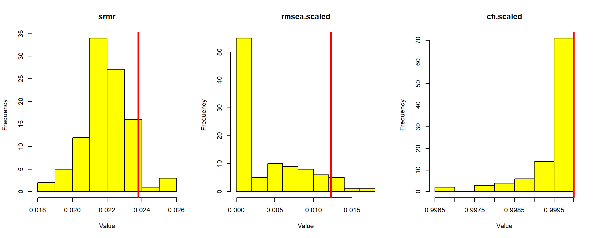
10.5 Sampling Distributions of Fit Indices
Figure 9 shows the empirical distributions of SRMR, RMSEA, and CFI across 100 replications, with rule-of-thumb cutoffs overlaid as vertical lines. The distributions should be concentrated well below (SRMR, RMSEA) or above (CFI) the cutoffs.
Figure 10: Sampling distributions of fit indices with simulation-based cutoffs at alpha = 0.05
10.6 Detailed Parameter Summary
The comprehensive parameter summary below reports, for each model parameter: coverage (proportion of 95% CIs containing the true value), power (proportion rejecting H₀: parameter = 0), relative bias in estimates, and relative bias in standard errors.
TipFull report simulation
To evaluate other parameters, such as the population value (true), mean estimate, standard deviation of estimates, mean standard error, etc., consider the command below:
Only few threshold parameters show power below .80 (see full report), and thresholds are generally not parameters of interest in CFA. All factor loadings and factor correlations are estimated with adequate power, indicating that the sample size is sufficient for reliable parameter estimation.
TipHow to Read the Parameter Summary
Key benchmarks for evaluating simulation quality (Rogers, 2024):
Power > .80: Adequate power to detect non-zero parameters
Coverage 0.91–0.98: Confidence intervals perform as expected (neither too liberal nor too conservative)
Relative Bias < |0.10|: Parameter estimates are unbiased (within 10% of true values)
Relative SE Bias < |0.10|: Standard errors accurately estimate sampling variability
Parameters outside these ranges deserve attention. However, thresholds are generally not parameters of interest in CFA. The focus should be on factor loadings, factor correlations, and residual variances.
The simulation results confirm that the sample size of N = 1047 provides adequate power for estimating all parameters of substantive interest. Factor loadings and correlations are estimated with power > .80, coverage near .95, and negligible bias. This supports the reliability and generalizability of the CFA results presented throughout this tutorial.
11 Summary and Conclusions
This supplementary material demonstrated a complete CFA workflow for ordinal data using the WHOQOL-BREF instrument, implementing the best practices described in Rogers (2024):
Data preparation (Section 3): Loaded data directly from Mendeley Data repository, verified structure and descriptive statistics
Population model (Section 4): Defined a teaching example based on Lin & Yao (2022) with analytically derived residual variances and equidistant thresholds
Model specification and estimation: Tested four competing structures:
Original 4-factor model with all 24 items (Section 5)
Bifactor model with general QOL factor (Section 6)
Revised 4-factor model excluding problematic item Q5 (Section 8)
Model evaluation: Applied DWLS estimation appropriate for ordinal data, examining overall fit (SRMR, RMSEA, CFI), local fit (MI, residuals), reliability (alpha, omega, AVE), and path diagrams
Model comparison (Section 9): Systematically compared all models, recommending the revised 4-factor model
Power analysis (Section 10): Assessed statistical adequacy via Monte Carlo simulation
ImportantKey Findings
Always use appropriate estimators for ordinal data: DWLS/WLSMV operates on polychoric correlations and does not assume normality of observed variables — using ML with ordinal Likert data leads to biased estimates
Item Q5 is systematically problematic across multiple model structures and should be excluded
The revised 4-factor correlated model (without Q5) provides the best balance of fit, interpretability, and statistical properties
Bifactor models improve fit mechanically but impose strong orthogonality assumptions that rarely hold; they should not be preferred solely on the basis of fit indices
All four domains show adequate reliability (omega > .70) in the recommended model
Sample size N = 1047 provides adequate power for all parameters of substantive interest
Examine both overall and local fit — global indices can mask specific, actionable problems
Modification indices should guide, not dictate: Only make theoretically justified changes, and be alert to items that appear repeatedly in high MIs
Lin, L.-C., & Yao, G. (2022). Validation of the factor structure of the WHOQOL-BREF using meta-analysis of exploration factor analysis and social network analysis. Psychological Assessment, 34(7), 660–670. https://doi.org/10.1037/pas0001122
McNeish, D. (2023). Dynamic Fit Index Cutoffs for Factor Analysis with Likert, Ordinal, or Binary Responses. PsyArXiv Preprints. https://doi.org/10.31234/osf.io/tp35s
Rogers, P. (2021). Data for "Best Practices for Your Exploratory Factor Analysis: A Factor Tutorial" [dataset]. In RAC-Revista de Administração Contemporânea. Mendeley Data, V2. https://doi.org/10.17632/rdky78bk8r.2
Rogers, P. (2024). Best practices for your confirmatory factor analysis: A JASP and lavaan tutorial. Behavior Research Methods. https://doi.org/10.3758/s13428-024-02375-7